Machine Learning for Financial Market

About this Project

This is a one-year compulsory final project for obtaining B.Eng Information and Communication Engineering from a Faculty of Engineering, Chulalongkorn University, Thailand. It is done in a group of three people, consisting of

1. Sivakorn Lerttripinyo (which is me!)
2. Krittapasa Boontaveekul
3. Wirachapong Suwanphibun

This project is graded by three faculty members, including one project advisor and two committees.

1. Advisor : Assoc. Prof. Chotirat Ratanamahatana, Ph.D
2. Committee Member : Asst. Prof. Kunwadee Sripanidkulchai, Ph.D
3. Committee Member : Lect. Aung Pyae, Ph.D

This blog will explain this project in an informal way, and in-depth details will be omitted. My main responsibility in this project is to design and implement the system component, which is the infrastructure and system for supporting the machine learning experiment. Therefore, this blog will mainly focus on the system component. The model training component, which is about how to do a feature engineering, choose and tune the ML algorithms, and evaluate the training result, will be briefly explained.

Although this project has already been concluded, this blog is not finished yet. Unfinished part in this blog will be filled with --Underconstruction--. However, you can read the slide I (and my friends) used for presenting the project here.

A Concise Informal Project Summary

As part of our B.Eng Thesis project, our team of three successfully implemented an End-to-End machine learning system for the financial market. The project has two primary components: operational implementation, guided by Microsoft MLOps standards, and model experimentation aimed at training robust models. Although we focused on cryptocurrency data, the concepts are broadly applicable to other financial products and fields.

We utilized AWS and DigitalOcean as our cloud providers. Almost all infrastructure under these cloud providers were managed by Terraform, which the state file was stored in S3; and DynamoDB was applied to do the state file’s lock management. Data ingestion was automated via Lambda and EventBridge Rules, while data transformation used ETL pipelines using Mage.ai as a data pipeline tool. MLFlow, hosted on an EC2, managed our model experiments. Experiment data and models are stored in RDS PostgreSQL and S3. Model performance was monitored through a Streamlit dashboard. APIs for serving the selected model were automatically built as a Docker image using BentoML and GitHub Actions and deployed using DigitalOcean’s App Platform. Notably, the MLFlow Alias feature allowed us to change the deployed model without rebuilding the image.

Our model experimentation involved minute-scale training data. After performing a feature engineering, closing price, SMA, and SMA differences were used to train the model. We applied various machine learning algorithms and evaluated the model performance using MSE and classification reports.

The final outcome was a functional E2E machine learning system, adaptable to other use cases. While the best model we can achieve didn’t perform as robustly as intended, they successfully captured price trends. The system leverages free-tier services, making it accessible for companies with limited budgets. Therefore, organizations starting to use machine learning can use our project as a guideline to implement the systems according to their needs.

Project Background

In the investment field, many people collect a set of history prices to analyze them to make a trading decision. For example, history prices of Bitcoin are collected to predict if the price is going to increase or decrease.

There is an idea that the computer maybe able to predict the price trend of these financial products by learning from the historical data, so a machine learning becomes more popular tools. If a robust model that can precisely predict the price trend can be trained, it will create a lot of profit to the user.

However, implementing a robust machine learning model is, in fact, not a simple task since training the model does not involve only a training step. The model training is only a part of the entire machine learning system.

• A data collection and processing is required to be a reliable data source for training the models.
• Infrastructures, such as VMs and databases, is required for implementing a system.
• A configuration to train each model (such as a set of hyperparameters) should be recorded along with each trainded model.
• A system to manage the deployed is essential since we are going to train a lot of models.

So, this project is intended to design and implement the system going beyond the machine learning experiment. The system will show the system for ingesting and preparing data; systematically tracking the conducted experiments and storing related metadata including but not limited to training results, hyperparameters, and models; and deploying selected version of model to the real-world application.

This project chooses to use cryptocurrency data to implement the system, but it can be easily adapted to be used with other financial products, such as a stock price, as well. I mean the system is the same, but you just only need to change the dataset.

Overview of this Project Structure

This project consists of two main components.

1. System Component, which is about how we design the system.
2. Model Training Component, which is about how we do a feature engineering, choose and tune the ML algorithms, and evaluate the training result.

System Component

Design Requirements

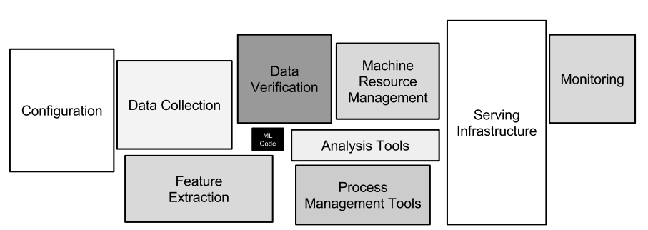
A machine learning system that targets for a model deployment involves the following steps.

• Data Extraction
• Data Analysis
• Data Preparation
• Model Training
• Model Evaluation
• Model Validation
• Model Serving
• Model Monitoring

I use MLOps maturity model to evaluate how much MLOps principles and practices are applied into the system. There is no standardized maturity model, but there are proposals from Google and Microsoft. For Google, the maturity level can be determined by the level of automation of these components. For Microsoft, the maturity model is evaluated by the technical capability.

This project attempts to achieve features from Microsoft’s MLOps Level 2: Automated Training. Some requirements are as below.

• A data pipeline automatically gathers data.
• Experiment results are tracked.
• Both the training code and the resulting models are version-controlled.
• The models are released manually, which are managed by software engineering team.
• Implementing models are heavily reliant on data scientist expertise.
• Application code has unit tests.
• Basic integration tests exist for the model.

Infrastructure as Code (IaC)

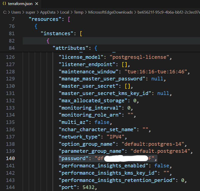
Most infrastructures used in this project are provisioned through running Terraform scripts. Scripts are stored in the GitHub so that all people in the project can collaborate on.

Terraform generates a state file to manage infrastructures and configurations. With its default configuration, the state file is generated and stored in a local machine. However, it should not be stored and managed by using GitHub due to reasons as follows.

• Manual Error: Any collaborator in the project can forget to pull down or push up the latest state file. As a result, any person can accidentally run Terraform with the outdated state file.
• Lack of Locking: Multiple collaborators may accidentally simultaneously run terraform apply on the same state file.
• Lack of Secret Management: All data in the state file is stored as a plain text, which is dangerous for storing sensitive data.

So, the Terraform state for this project is managed by using Terraform’s built-in support for remote backends instead. The Terraform backend is responsible for loading and storing state, and the remote backend is used to store the state file. AWS S3 is chosen to be the remote backend, and AWS DynamoDB is chosen to manage the state locking.

Although requiring to have more infrastructures to only manage Terraform seems troublesome, it allows the collaboration on managing the infrastructure from other members, and the state is safely stored and managed. Moreover, both S3 and DynamoDB are covered by AWS Free Tier. So, only little additional cost incurs after 12 months for the AWS S3. DynamoDB’s free tier lasts forever if the usage does not exceed the limit.

Database

The main purpose of this system is to provide a clean and reliable source of data for conducting the model experiment and being used by other components.

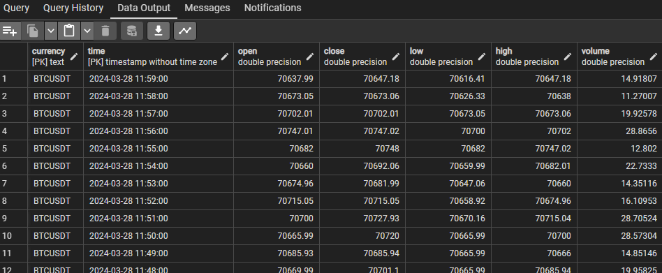
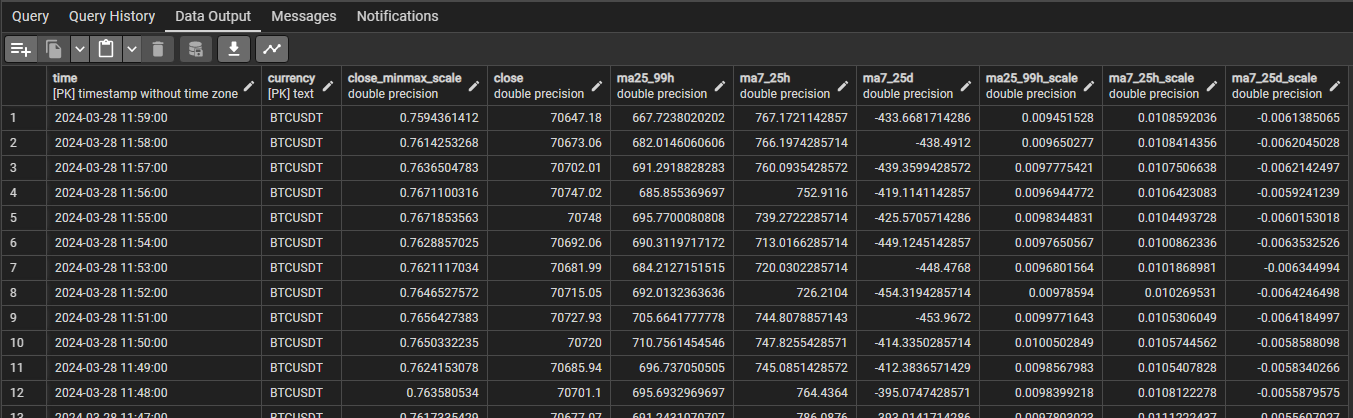
There are two types of data consisting of raw data and derived data. Raw data is ingested from external systems through various channels such as APIs and CSV files. For this project, the raw data is mainly a set of datetime and price of each currency. For example, raw data is a set of closing prices, opening prices, and volumes of BTCUSDT from 28 Apr 2019 to 31 Jun 2023. Derived data is the data that is derived and transformed from the raw data. For example, a moving average(MA) price can be derived from a set of closing price from a specific currency.

For raw data, the attributes are fixed, which are datetime, currency name, open price, close price, highest price, lowest price, and volume. Duplicate data in the storage is not allowed as one datetime and one currency must have only a single set of data. After considering the requirements, a relational database is chosen as it can handle fixed schema, prevent duplicate data by applying a primary key as (datetime, currency), determine a data type for each attribute, and enforce constraints such as NOT NULL easily.

The design for storing derived data is one table for each model. When deploying the model, each model can use different set of indicators. For example, one model may use MA 5 minutes and MA 7 minutes as indicators, while another model may use MA 30 minutes and MA 60 minutes as indicators. So, the decision is that each model uses data from each own table. Although there is a scenario that two models use the same indicator, they are stored redundantly in both tables. Therefore, each table has a fixed schema. The relational database is chosen to store the derived data.

PostgreSQL hosted on AWS RDS is chosen to be the database server. The database provisioned here is further used in other parts of the project as well.

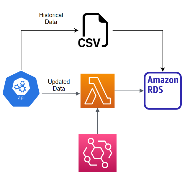
Data Ingestion

Raw data is ingested and inserted in two approaches including historical data and new data. Historical data ingestion is performed to a new currency data that is not already available in the database. After that, newly-generated data needs to be inserted periodically to keep the data in the database updated.

Historical data, which is a historical price of a particular currency, is inserted manually because it is an only one-time operation and involves a large amount of data. The dataset can be downloaded, and a bulk insertion can be performed instead of having the automated system to perform a loop to insert data row by row. The bulk insertion is more efficient and consumes less time to insert all historical data.

The automation system is implemented to automatically insert newly-generated data, which is smaller than the historical data, into the raw-data database. This system can eliminate the work to manually keep the data in the database up-to-date.

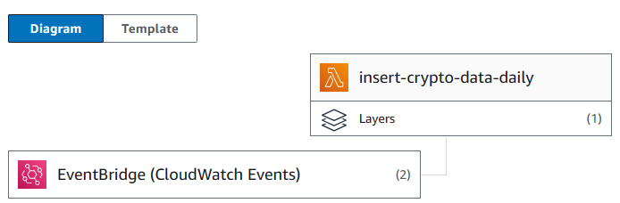
AWS Lambda is chosen to implement the data ingestion system. The function, which hosts the script, does not need to be working all of the time. It is designed to be triggered only at a designated point of time. So, AWS Lambda is an appropriate service as no instance has to be provisioned and run at all time. AWS EventBridge rule is used to trigger the function at a specified time.

However, managing dependencies in Lambda is difficult. If the script requires libraries not included in the environment, the layer containing necessary libraries must be manually created and inserted into the function. Therefore, AWS Lambda can be an inappropriate tool for performing operations requiring several extra dependencies.

For the data ingestion, the function requires only receiving new data, performing a schema mapping between a response and the table in the database, and inserting into the table. However, for the data transformation, many complex transformations may be performed before storing into the database. Using AWS Lambda environment can be difficult to test and debug the function. So, finding data pipeline tool can be more suitable for the higher transformation workload.

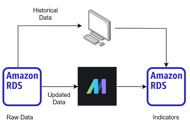
Data Transformation

Deriving and storing indicators from the historical data is done manually. Raw data is queried from the raw-data database and simultaneously derived into all indicators. Finally, the indicators are stored in the database. The reason this operation is done manually is that it is a one-time operation that involves a large amount of data. Million rows of historical raw data can be involved in the process of deriving indicators. Configuring the tool for supporting a processing of the large chunk of data, which runs only one time, is not worthwhile.

However, newly-generated data is automatically queried, transformed, and stored. Because this operation can involve complex data transformation, data pipeline tool is utilized instead.

Apache Airflow is one of the first tools that people may think of; however, it is inappropriate for a small project for a reason. Although Airflow provides a lot of features and allows a lot of customization, the learning curve for using it is significant. Moreover, it requires a high specification of the instance to host on to work properly, and it is difficult to set up. This tool is worth using for larger projects.

Therefore, a simpler tool, Mage, is considered. In a nutshell, Mage is a tool for creating data pipelines. This tool requires less infrastructure specification, and it is easy to install and use. Its functionality is less than Airflow, but it contains all necessary features for a smaller project size.

This is an example of the data pipeline implemented in Mage. The pipeline contains several blocks connected with each other as a directed acyclic graph(DAG).

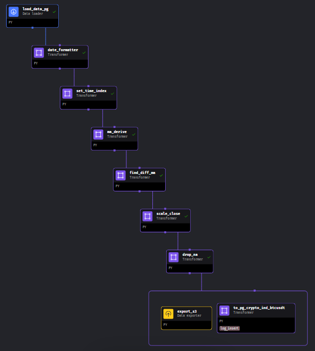
Mage includes a unit test capability to each block. So, the unit test can be implemented in each block to ensure that it works as intended. For example, the following code is one of the blocks in the data pipeline used to derive moving average indicators. There are two testcases included, which the test functions are decorated by @test. If there is any value contradicts the intended value, the testing function returns an error, which causes the pipeline to be failed. According to the code snippet, it validates whether the function df_ma_x_hour and df_ma_x_day provides the correct result and check whether the output of this block is not None.

# <omit previous unrelated code>

def df_ma_x_hour(inp_df, window_size, col_name, round_decimal=10, idx_name='time'):
    df_ma_x_h_p = inp_df.groupby(inp_df.index.minute).rolling(window=window_size)[col_name].mean().round(round_decimal)
    df_ma_x_h = df_ma_x_h_p.droplevel(0).reset_index().set_index(idx_name).sort_index()
    return df_ma_x_h

def df_ma_x_day(inp_df, window_size, col_name, round_decimal=10, idx_name='time'):
    df_ma_x_d_p = inp_df.groupby([inp_df.index.hour, inp_df.index.minute]).rolling(window=window_size)[col_name].mean().round(round_decimal)
    df_ma_x_d = df_ma_x_d_p.droplevel([0,1]).reset_index().set_index(idx_name).sort_index()
    return df_ma_x_d

def generate_dataframe_hour(x_hours: int):
    dt_range = pd.date_range(start="2023-01-01", periods=x_hours*60, freq='T')
    values = range(1, len(dt_range) + 1)
    df = pd.DataFrame(data=values, index=dt_range, columns=['close'])
    return df

def generate_dataframe_day(x_days: int):
    dt_range = pd.date_range(start="2023-01-01", periods=x_days*24*60, freq='T')
    values = range(1, len(dt_range) + 1)
    df = pd.DataFrame(data=values, index=dt_range, columns=['close'])
    return df

@transformer
def transform(df, *args, **kwargs):
    df_ma7h = df_ma_x_hour(inp_df=df, window_size=7, col_name='close', idx_name='time')
    df_ma25h = df_ma_x_hour(inp_df=df, window_size=25, col_name='close', idx_name='time')
    df_ma99h = df_ma_x_hour(inp_df=df, window_size=99, col_name='close', idx_name='time')
    df_ma7d = df_ma_x_day(inp_df=df, window_size=7, col_name='close', idx_name='time')
    df_ma25d = df_ma_x_day(inp_df=df, window_size=25, col_name='close', idx_name='time')
    return [df, df_ma7h, df_ma25h, df_ma99h, df_ma7d, df_ma25d]

@test
def test_output(output, *args) -> None:
    assert output is not None, 'The output is undefined'

@test
def test_func_ma_finder(output, *args) -> None:
    test_h = generate_dataframe_hour(7)
    res_test_h = df_ma_x_hour(inp_df=test_h, window_size=7, col_name='close', idx_name='index').dropna()
    assert np.isclose(res_test_h.iloc[0],181.0)[0], "df_ma_x_hour may provides a wrong result"
    test_d = generate_dataframe_day(7)
    res_test_d = df_ma_x_day(inp_df=test_d, window_size=7, col_name='close', idx_name='index').dropna()
    assert np.isclose(res_test_d.iloc[0],4321.0)[0], "df_ma_x_day may provides a wrong result"

Training Management System

The purpose of this system is to track experiments, record relevant information, and be a central position for distributing models. MLFlow is a tool that fits the requirements as it focuses on the entire lifecycle of machine learning projects, ensuring that each phase is manageable, traceable, and reproducible.

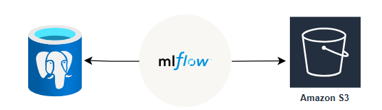
MLFlow is hosted on an AWS EC2 instance. To use it to track experiments, destination for storing a backend store, which stores metadata for each run and experiment, and an artifact store, which store artifacts for each run such as model and data files, must be configured. Initially, its default value is the local device, which is the instance used for hosting MLFlow; however, if any failure occurs to the instance, all data can be lost. Therefore, configuring MLFlow to store metadata and artifact to other appropriate location is a better choice. PostgreSQL and AWS S3 are used to store metadata and artifacts of MLFlow, respectively.

Here is the example of the code snippet for training and logging the model into MLFlow.

TRACKING_SERVER_HOST = "..."
mlflow.set_tracking_uri(f"http://{TRACKING_SERVER_HOST}:<port>")
mlflow.set_experiment("...")
with mlflow.start_run(run_name="..."):
    params = {
            "colsample_bytree": 0.3,
            "learning_rate": 0.1,
            <more params can be added>
        }
    mlflow.log_params(params)
    xg_reg = xgb.XGBRegressor(**params)
    xg_reg.fit(X_train, y_train)
    y_test_pred = xg_reg.predict(X_test)
    test_mse = mean_squared_error(y_test, y_test_pred)
    mlflow.log_metric("test_mse", test_mse)
    mlflow.xgboost.log_model(xg_reg, "model")

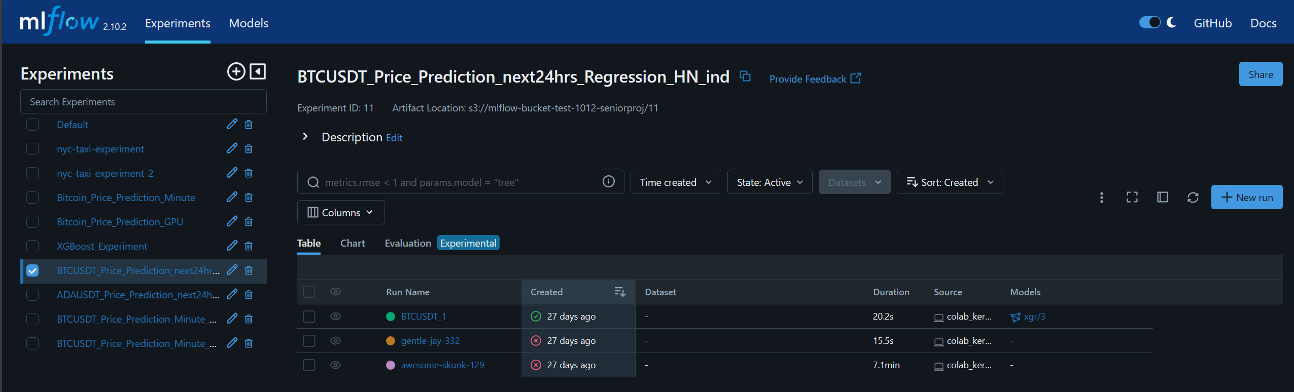
The experiment information is recorded to MLFlow. From the example, there are three runs in this experiment.

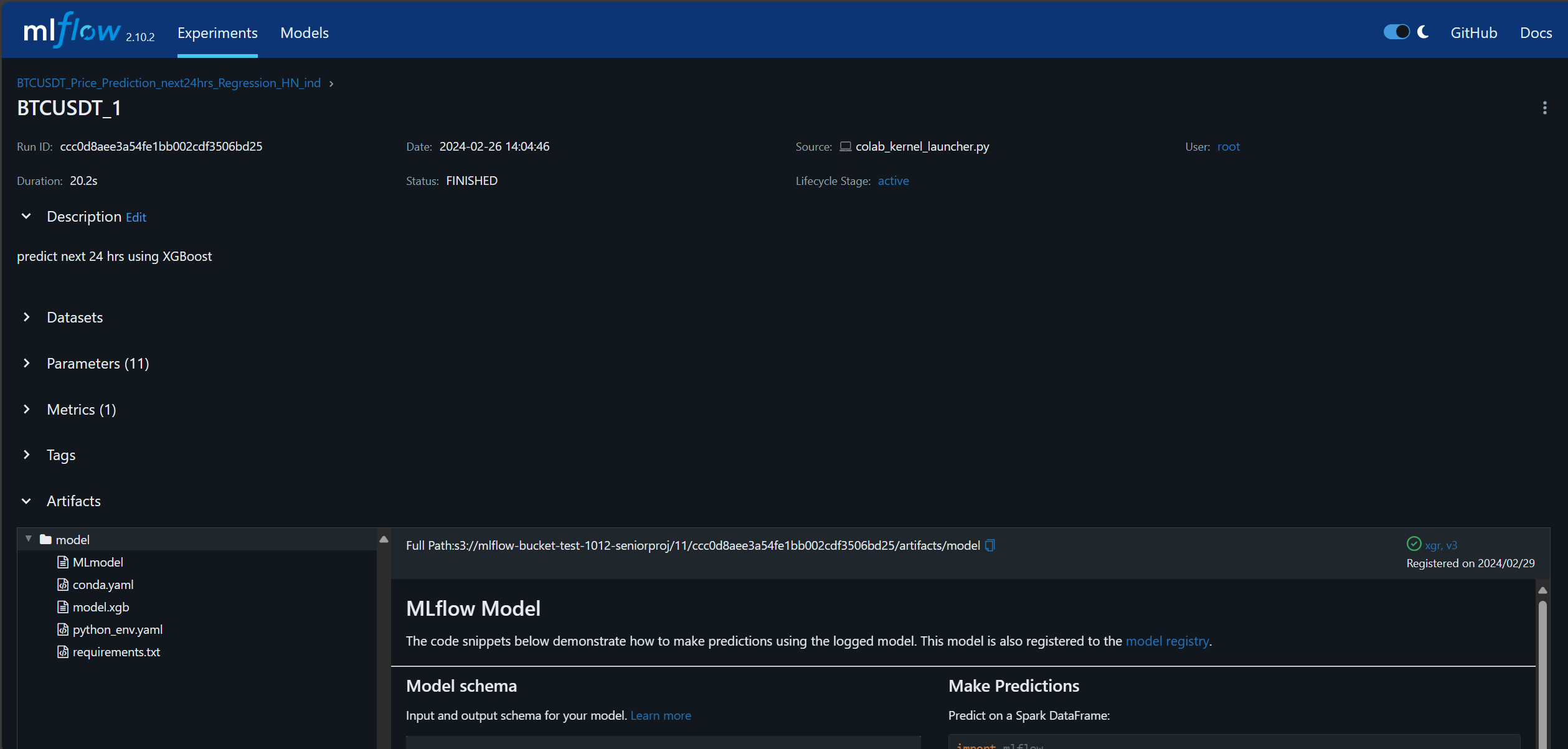
This is the details of one of the runs named BTCUSDT_1.

Model Monitoring

To continuously monitor the model performance, all related metrics and graphs are needed to be plotted and displayed. Although creating a Jupyter notebook to do this task is possible, it can be inconvenient to open it every time to monitor the performance. It can be more convenient if there is a webpage to show all related metrics and graphs. Only opening the webpage by inputting the URL to the browser from anywhere and any device can be more simple than opening the notebook from only the computer. Moreover, sharing the URL to other people is easier than sharing the Jupyter notebook.

The main requirement for this webpage is to display metrics and graphs. Because of the simple usage, a complex library or framework, which requires high learning curve and high amount of implementing time such as React and Angular, is unnecessary. Streamlit is chosen because it uses Python, which is the programming language already used in this project, and it is well integrated to visualization libraries, such as Matplotlib. The webpage is hosted on the instance and set to be able to be accessed by any browser.

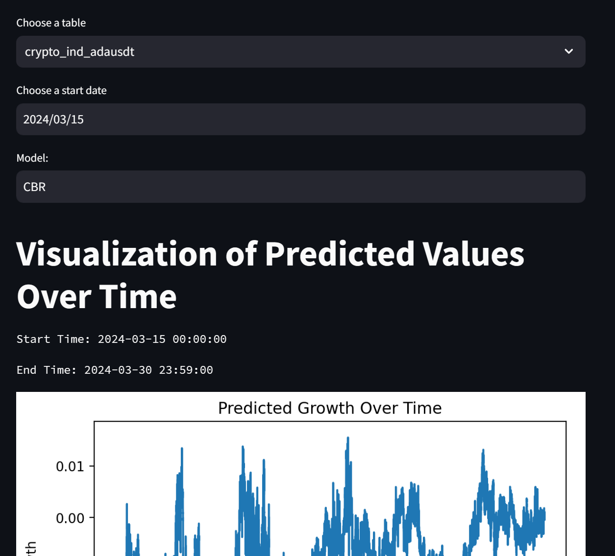
The webpage visualizes the performance of the model. The user can customize the currency to evaluate, the start datetime for evaluation, and the model algorithm. The result shows the start and end datetime of the evaluation, the predicted growth, the comparison between the predicted growth and the actual growth, and the MSE value calculated from this data using the specified model.

Model Building and Serving

Deploying the model to an application is not a trivial task. In order to connect the gap between the model and the application, the intermediate format containing all model dependencies is required so that the model can be run in this environment. Therefore, the process for serving the model is separated into two parts including building and deploying, respectively.

An intermediate artifact should be an object that all dependencies are packed and ready to be deployed. The tool chosen to help build this artifact is BentoML. The following figure summarizes the model building and serving system.

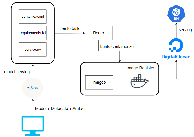
The model serving APIs are implemented in service.py, which retrieves the models from the MLFlow. The bentofile.yaml is used to define required dependencies and python scripts to be bundled into the intermediate artifact. These files are then used to build the bento through the BentoML command line interface. bento is the intermediate artifact which prepares all necessary environments for running the model and locks the version of API service to be easily converted into a docker image. It can be used to serve the APIs service when the necessary dependencies are installed in the environment. For the ease of deployment, the bento is then converted into a docker image through the BentoML containerize command.

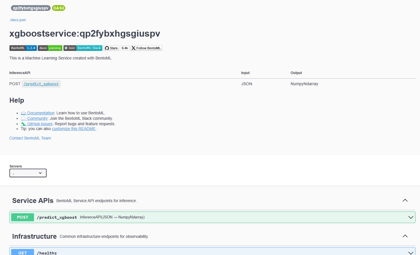
The DigitalOcean App platform is utilized to deploy the service. The image is built and stored in an image registry provided by DigitalOcean. App platform retrieves the image to deploy the service automatically from this registry. Deployed APIs can be tested through an autogenerated Swagger UI, which is accessed by a link provided by App.

Finally, performing these steps, starting from building bento to pushing the image into the image registry, manually can be a tedious task and error-prone. Therefore, they are automated by implementing a GitHub workflow script to trigger GitHub action to automate them when there is any commit updated into the main branch. Three files used to build the bento are initially stored and edited in another branch in GitHub. After passing the local testing, it is merged into the main branch to trigger the automation.

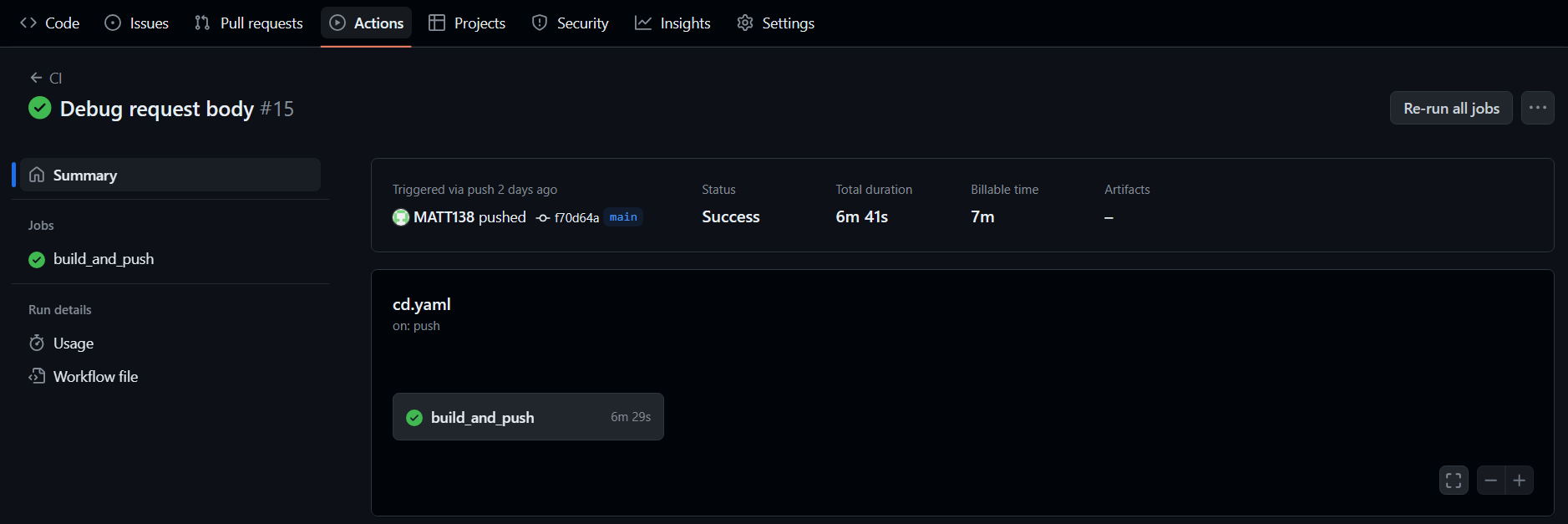
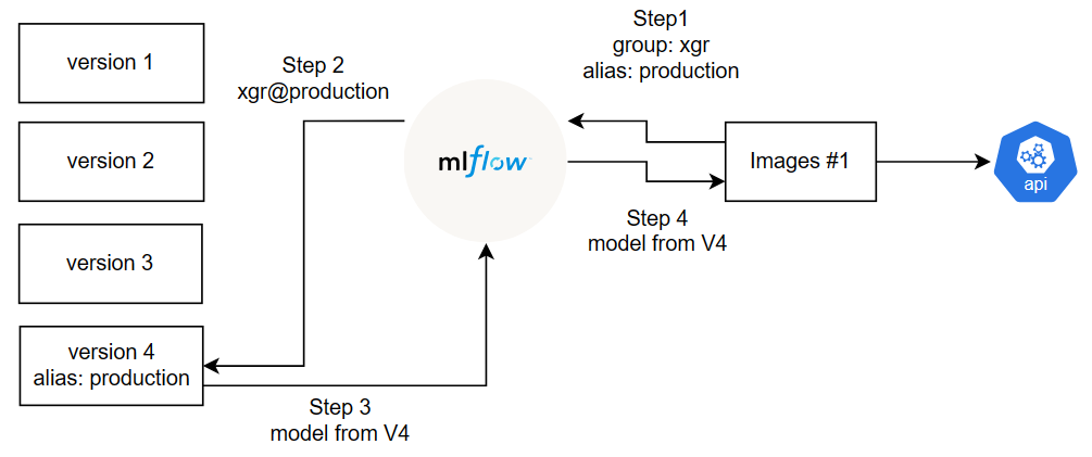
However, it is inefficient to rebuild the image and redeploy every time the new model is selected although the automation is implemented since all processes requires at least six minutes. Alias concept, which is a feature of MLFlow Model Registry, can solve this problem.

Models can be registered as a version within a group.

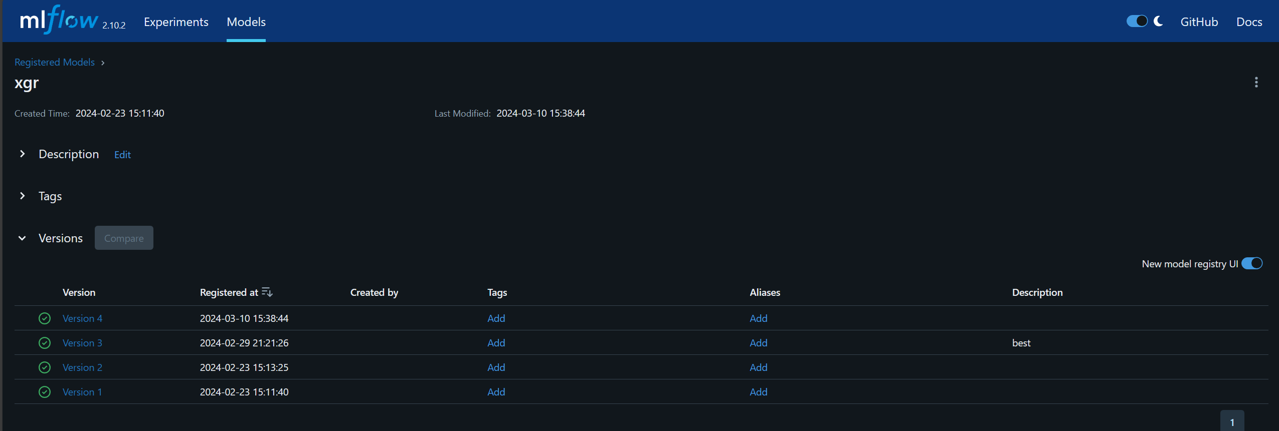
For this example, four models are registered in xgr group as four different versions. The alias can be assigned to a particular model. The model can be retrieved by specifying the group name and alias name.

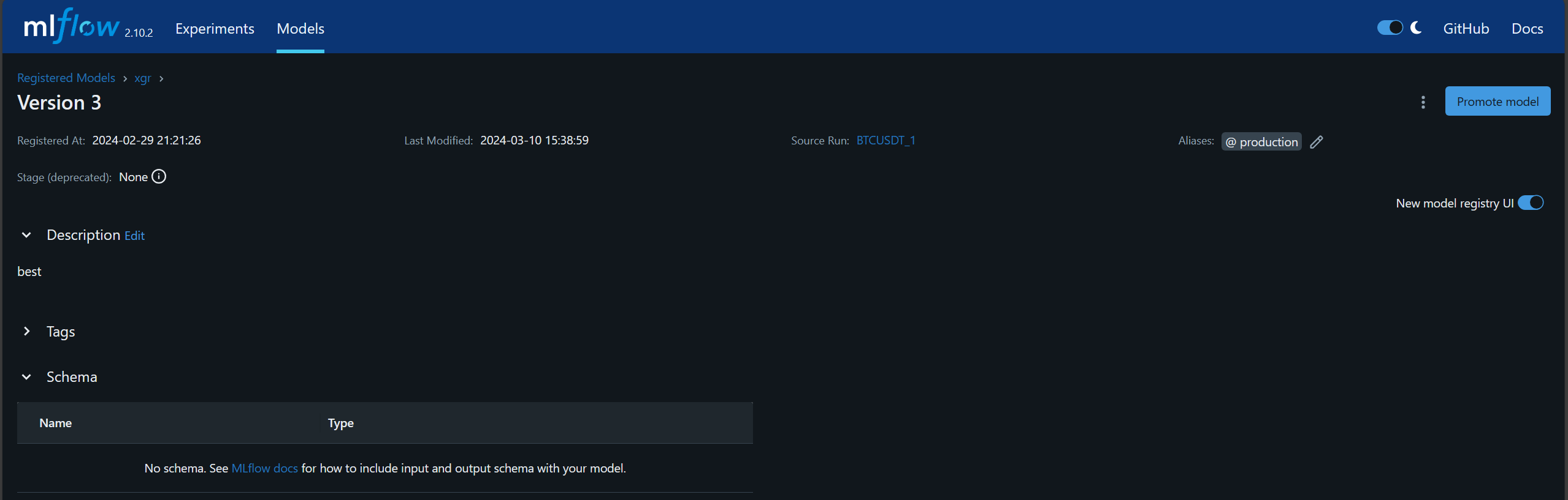
the production alias is assigned to the model version 3 of xgr group.

The model can be retrieved by using the URI models:/{group-name}@{alias}, such as models:/xgr@production. MLFlow has a function mlflow.pyfunc.load_model(URI) to load the model.

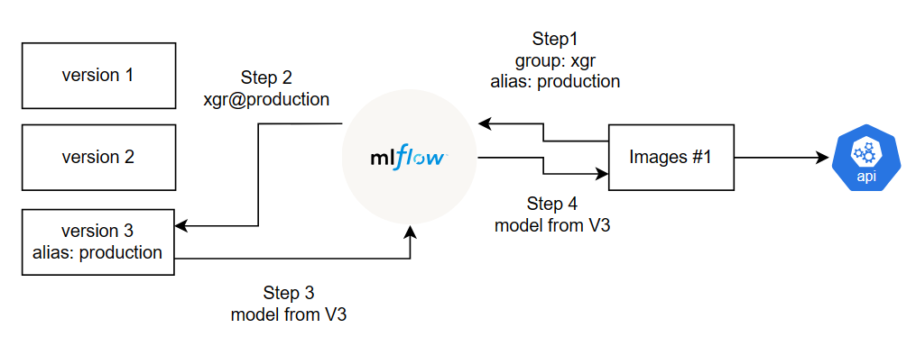
If there is a better model available, it can be registered as a new version in the group, such as being a version 4 in xgr group. The production alias can be given to the new version instead. When the application requests the model with production alias in xgr group, MLFlow automatically retrieves the version 4 of the model and sends it to the image. As a result, the new model is applied and served without rebuilding the new image and container.